We built a shared-memory parallel aggregate and measured what it buys — and what it costs

In this article written for experienced PostgreSQL engineers and core developers, I want to describe how we tested one hypothesis — whether a shared hash table can be used to speed up parallel aggregation by hashing. A recent paper claims that the shared hash table is an unfairly dismissed way of doing parallel aggregation, and that the key to success is moving the group lookup out from under the lock. We considered the idea of shared parallel aggregate, brought it to a working patch set for PostgreSQL, and ran measurements on a many-core instance in Google Cloud.

The questions I wanted to answer:

1. Does the hypothesis hold in PostgreSQL — and if it does, how exactly.

2. What we pay for it.

3. Is contention on LWLock really the only bottleneck?

4. Can this approach be reused to speed up other operations in a query plan?

The short answer to the third question: no, it is not the only one. The lookup under the lock is the biggest of the problems, and it can be removed. Underneath it we found at least three more issues (two of which are invisible in the paper), because it is written about an engine with threads rather than processes.

The starting point

From time to time I get reports from PostgreSQL users complaining that a query which looks quite simple takes a very long time. EXPLAIN ANALYZE in such a case looks roughly like this:

Finalize HashAggregate (actual time=22022.997..24117.957 rows=592000.00 loops=1)
   Group Key: f008_type, f008_rtref, f008_rrref, f009rref, ...
   Batches: 1  Memory Usage: 4481049kB
   ->  Gather (actual time=2024.452..6237.613 rows=2440146.00 loops=1)            
         Workers Planned: 8
         Workers Launched: 8
         ->  Partial HashAggregate
             (actual time=2018.297..4047.409 rows=271127.33 loops=9)
               Group Key: f008_type, f008_rtref, f008_rrref, f009rref, ...
               Batches: 1  Memory Usage: 1949721kB
               ->  Parallel Seq Scan on bench_shagg_num
                   (actual time=0.160..252.678 rows=333333.33 loops=9)
 Planning Time: 0.839 ms
 Execution Time: 25071.708 ms

Here we see an ordinary table scan and an aggregate over the result. The scan takes a negligible amount of time (250 ms), the partial aggregate fits into four seconds, Gather delivers rows by the sixth — and after that, about 18 of the 25 seconds are eaten by Finalize, which runs in a single process. Everything happens in memory, so spilling has nothing to do with it. The aggregation is done by hashing, so no hidden sorts are expected either.

Part of the reason is visible right here: 3 million rows on the input, almost 600 thousand groups on the output. Five rows per group means that the partial aggregation barely compresses the data stream, the hash table grows fat both in the workers and in the leader, and about 2.44 million partial states are sent through Gather.

The second part can be seen in the query itself:

SELECT
    f008_type, f008_rtref, f008_rrref, f009rref, f010rref,
    f011_type, f011_rtref, f011_rrref, f012, f013rref,
    f014rref, f015rref, f016rref,
    SUM(v1), SUM(v2), SUM(v3), SUM(v4), SUM(v5), SUM(v6), SUM(v7)
FROM <table>
GROUP BY
    f008_type, f008_rtref, f008_rrref, f009rref, f010rref,
    f011_type, f011_rtref, f011_rrref, f012, f013rref,
    f014rref, f015rref, f016rref;

The grouping is done on thirteen variable-length fields from the middle of the table, which tells us that the hashing is probably unusually expensive. And seven SUM(numeric) processes are not a cheap operation either, keeping in mind the number of rows processed. On top of that, Finalize actually redoes all the work on the keys: every state emitted by the Gather node has to be hashed again and compared on the same thirteen fields, and the aggregates have to be computed.

Without workers, this query behaves better:

HashAggregate (actual time=10392.242..12376.055 rows=592000.00 loops=1)
   Batches: 1  Memory Usage: 4481049kB
   ->  Seq Scan on bench_shagg_num 
       (actual time=0.015..831.849 rows=3000000.00 loops=1)
 Execution Time: 12958.788 ms

The parallel plan is almost twice as slow as the serial one. The effect of such a “cure” is limited, and the question remains how to make this decision by cost.

How it could be arranged

Let us try to imagine the possible ways of parallelising the aggregation:

1. Row routing — before aggregating, the tuples are distributed among the workers according to a hash function on the grouping condition, that is, “partitioning”.

2. Merging partial states — the current Partial/Finalize implementation.

3. A common “shared” aggregation table.

4. Routing of grouped states — do the “partial” aggregation independently, but redistribute the values among the workers before merging.

5. Private accumulation with a flush into a shared table — a combination of the “partitioned” and “shared” options (a hybrid of options 1 and 3).

Option 5 looks interesting, if we ignore how hard it is to implement. But what do relational DBMSs actually use today?

The Industry Standard

In my experience, SQL Server usually employs the Parallelism (Repartition Streams) operator with a hash distribution by groups. The rows of one group are guaranteed to land on a single thread, after which each thread computes its own Hash Aggregate independently and in full. No final regrouping is needed, which ideally can give scaling close to linear. Oracle and Greenplum apparently follow the same pattern. DuckDB chose option 4. HyPer does a variation of the same — thread-local pre-aggregation, then a partitioned merge phase where each thread takes ownership of its own partitions (Leis et al., Morsel-Driven Parallelism, SIGMOD 2014).

In PostgreSQL, however, with its model of independent worker processes and a single Gather at the end, there is nothing like this. In principle, it is fairly easy to invent, with an extension module, a custom “SPLIT” node that redistributes rows among the workers according to the hash value of the grouping attributes and offers the optimiser an alternative plan, something like this:

Gather
  Parallel Aggregate
    Parallel Split
	  Parallel Scan <table>

The approach is good — in fact nothing has to be changed, the aggregate functions work as they are. However, attempts to do this run almost immediately into the question of load balancing and into the data skew that is unavoidable in real life, which, with independent processes, almost cancels out the effect of parallelism. And introducing threads is too invasive and too unreliable.

Spilling to Disk as a Way of Repartitioning

While looking for a Postgres-style implementation, it is worth glancing around. The first thing that comes to mind is the minimal option: repartitioning through spilling.

The idea exploits the fact that Postgres already has the machinery in place: when work_mem overflows, the HashAgg operator splits the input stream into batches by the hash of the grouping keys and dumps the “extra” ones into files. The question is whether the same machinery, driven not by memory but by the number of workers, can be used to build repartitioning for a parallel finalisation.

At first glance this approach can be implemented with minimal changes. A shared queue of buckets is added to the existing spilling code, with buckets picked up as workers become free. Correctness is ensured in the same way as in HashJoin: if the bucketing goes by the same grouping keys, then each group lands entirely in one bucket.

However, this approach introduces mandatory I/O even when the data fits fully in memory, which means a regression for the typical case: the example from the beginning of the post could become even slower, since no spilling was needed there at all. Secondly, this is two full passes over the data (writing into all the buckets, then reading from them). Finally, the skew does not go anywhere: the most frequent grouping key will settle entirely in one bucket, and a single worker will chew through that bucket alone — the same bottleneck as in the SPLIT option.

This may work as an improvement for the cases where the data does not fit in memory anyway (the spill is unavoidable) and at least some parallelism is needed at the Finalize stage; the path works and is cheap to implement. But as the main road to parallel aggregation it is not good enough.

Computing an aggregate in parallel on a shared hash table

Clearly, each method is good in a particular situation — see, for example, Adaptive Aggregation on Chip Multiprocessors, VLDB 2007 or Scalable Aggregation on Multicore Processors, DaMoN 2011. Option 4 is obviously good on a single powerful instance, option 1 is the basic way of doing shared-nothing parallel query processing, and the shared-table option should be as thrifty and as efficient as possible when there are no “heavy hitter” groups. But some of them are bound to fit the architecture of a particular DBMS better, and some worse. So we have to try.

A recent publication, Xue & Marcus, Global Hash Tables Strike Back! An Analysis of Parallel GROUP BY Aggregation, PVLDB, 2025, proposes an implementation with a shared table which, by their results, catches up with and overtakes partitioning on most workload profiles. The essence of the approach is that shared memory can be organised specifically for the aggregation task. The main trick of that specialisation is to separate the “find the group” and “update the state” operations by means of so-called ticketing, which removes the need for a heavy LWLock during the lookup.

The same paper also implies that the alternative modes of parallel aggregation have their own niche. And the choice between the strategies must be cost-based.

Building a prototype

So, in order to better understand the specific strengths and weaknesses of the shared approach in the Postgres architecture, as well as how invasive the solution is, we started a weekend project to implement it. Luckily, the capabilities of AI agents are now good enough for an experienced team to quickly produce code (in prototype form) that touches all the main architectural questions and is stable enough to survive the regression tests and heavy benchmarks.

For the sake of simplicity and development speed we decided to drop the ticketing idea for now, since even the authors of the paper themselves admit that this method has several open questions (spilling, for example).

The resulting parallel aggregation code can be found in a branch on GitHub.

What had to be written from scratch

The hash table. The first thing we had to do was give up the dream of reusing the shared hash table from parallel hash join (PHJ). A shared hash table for aggregation requires a lock, because unlike PHJ, where there is a split into insert/read phases, here the result of a table lookup is either an insert of a new element or an update of an existing one. This is where the further (rather complex) hash table optimisations come from — their goal is to reduce the effect of introducing locks. The authors of the paper come to the same conclusion: a join hash table is generally incompatible with the needs of fully concurrent aggregation.

The by-reference state layer. The Postgres core and the aggregate functions have a contract (see AGG_CONTEXT_AGGREGATE) saying that such a function may change the intermediate state of the aggregate (by calling repalloc, for example). The aggregate performs such operations outside the Dynamic Shared Memory Area (DSA) area given to it. Whether a particular aggregate does this or not is impossible to tell, since this property is defined by the implementation of the particular function. Parallel aggregation therefore had to be extended with a mechanism for copying out of shared memory beforehand and copying back afterwards (or allocating a new DSA). This concerns by-ref types such as numeric or text, and min /max over them.

Memory limit. The same feature of by-ref states also complicated the accounting of consumed memory, which is needed to understand when to switch to spilling. In the PHJ hash table, the granularity of accounting matches the granularity of allocation: memory is handed out in chunks, a tuple is put into a chunk and never changes size after that, so the shared counter is touched once per chunk and is always exact — it is updated under the same lock as the allocation. In our implementation this is only true for by-value states. A by-ref state can change size, so its blob cannot be handed out by the chunk allocator: that allocator can only allocate additively and free everything at once, while here individual allocate/free is needed. We solved this by accumulating the memory counter locally and publishing it into the shared counter in portions. Probably not the best solution.

Scope of application. A check of whether parallel aggregation is valid was added to add_paths_to_grouping_rel() for each particular aggregate type. The mechanism itself suggests that such an optimisation needs a new pg_aggregate flag, aggsharedsafe, set for each aggregate separately. It leaves an open question, though: how to control that this flag is assigned correctly. Apart from the safety of the aggregate itself, the optimiser must also check the grouping keys fed into such an aggregate.

The expression interpreter. For by-reference states, expression interpretation (ExecInterpExpr / ExecBuildAggTrans) cannot be used in its current form, and the shared path goes around it: the interpreted (or, with JIT, compiled) “microprogram” state ExprState produces the intermediate aggregate value in local memory, and references to it cannot be put into DSA. Expression interpretation for by-value aggregates can be done in the traditional way, but the evaluation of the expressions will still run under the LWLock.

What gets reused

Practically all the low-level machinery is used as building blocks in this code. SharedTuplestore — the whole of spilling, which the Xue & Marcus paper calls an open question, came almost for free.

All the phase synchronisation, the temporary files and DSA are used as they are. Five new wait events and two LWLock tranches were added to the core (following the Parallel Hash Join pattern) so that pg_stat_activity can tell the two different kinds of contention apart.

Adapted from an Existing pattern, but Written Anew

DSM management. The concurrency of the DSA allocator in PostgreSQL is still an open problem [1]. That is why, like Parallel Hash Join (PHJ), we do not go to DSA for every object, but build chunked placement on top of it. For aggregates with a by-value state each participant requests a 32 KB chunk and cuts records off it one after another as new groups appear; freeing happens in bulk, the whole chain of chunks at once. Aggregates with a mutable, by-reference state still call dsa_allocate/dsa_free, because the size of the state can change. The main optimisation here is rewriting in place: if the size of the new state has not grown, the DSA machinery is not used at all. For parallel aggregation this code is critically important, since memory management happens under the lock.

Partitioning rules when spilling. The flat partitioning scheme of PHJ applies to aggregation as well — it is a special case of the recursive one with a wide first level — but its code is tied to the hash join structures and would have to be written from scratch. So, since the in-core partial/finalize aggregation already has its own spilling mechanisms, we decided to go the same way and use the same recursive spilling scheme for shared parallel aggregate too.

The fundamental difference between aggregation and a join is that the amount of memory needed is determined by the number of groups, and that is not directly related to the number of rows. Fixing a maximum batch size is therefore pointless: the boundary is not the size, but the moment when the table, while processing a batch, hits the memory ceiling. From that moment the participants switch to spilling mode — existing groups keep being updated in place, while new ones go into child partitions.

At the same time, using the HyperLogLog machinery already present in the core, one can estimate both the cardinality of the next repartitioning step for a batch and the efficiency of that repartitioning: whether the number of groups in each particular batch drops significantly.

Barrier machinery. There is only one shared hash table here, and to keep the prototype simple the batches are processed strictly one after another. Hence the small number of barriers: build_barrier (the ELECT, ALLOCATE and BUILD events) and scan_barrier (the EMIT and BATCH events) — against three global barriers plus one per batch in Parallel Hash Join. This is not a saving but a consequence of less parallelism: at the boundary of every batch there are three global synchronisation points where everybody waits for the slowest participant, whereas the PHJ participants walk around the batches in a ring and pick up a free one without any common synchronisation. A better option could be implemented by merging small batches of one level into a single load (bucket tuning) — but that requires estimating the cardinality of the batches, which is out of the prototype's scope for now.

Changes in the subsystems

The overlap with the existing nodeAgg.c is small — eight static functions: fetch_input_tuple, prepare_hash_slot, select_current_set, finalize_aggregates, prepare_projection_slot, project_aggregates, build_hash_tables, hash_agg_check_limits. In principle, the parallel aggregate could be implemented in a separate module, nodeAggShared.c, with the shared machinery moved into a separate common module.

Outside nodeAgg.c about ~800 lines had to be changed, of which ~600 fall on the planner (the decision mechanism and the cost model) and ~60 on EXPLAIN. In other words, deciding whether the strategy is applicable and how much it costs turned out to be more expensive than all the rest of the integration with the plan tree put together.

The changes in the executor core amount to seven lines; one case of T_AggState is added to  ExecParallelReInitializeDSM and ExecShutdownNode_walker. The executor needed nothing more: the ExecParallel* mechanism turned out to be general enough for a new node to be added through the dispatching that already exists.

Testing

To find out the real effect of parallel aggregation, we made test runs on a GCP VM.

The measurements were taken in three rounds on different hardware:

• The first — 48 physical cores (c4-standard-96-lssd, Intel Granite Rapids, SMT off, two NUMA nodes of 24 cores each, 354 GB): that is where the main matrix was taken, the terms of the cost model were isolated and the first probes of locking and NUMA were made.

• The second — 16 physical cores (c4-standard-32, Xeon 8581C, SMT off, one NUMA node, 118 GB): all the rounds from the “Testing” section, except those marked separately.

• The third — a 14-core laptop, where the Zipf profiles missing from the first two rounds were measured. Absolute times from different rounds must not be mixed; ratios within one round are comparable.

A couple of ground rules for our testing:

1. Only the plan for the parallel aggregate case and the number of workers in the plan are forced (by minimising the costs). In the base case the optimiser itself decides whether to use serial hash aggregation or the Partial/Finalize approach with workers.

2. shared_buffers and work_mem are large enough that during the query neither the scan nor the aggregation needs to read data pages from disk or to spill.

In light of the limitations these tests cover only aggregates without an “Internal” state, like sum(numeric).

Results

On the graphs below, the “speedup” exposes the relation between query execution time picked by the optimiser from the current master branch and patched parallel aggregation. The choice of the current Postgres is defined by the cost model. Parallel aggregate is forced.

The first result is a positive one (fig. 1). With values spread evenly across the groups, we see a clear advantage of parallelising with a shared table over the current state of things. Aggregates with a fixed-size state obviously show better numbers than those which need extra copying out of and into shared memory, but even 2x is encouraging.

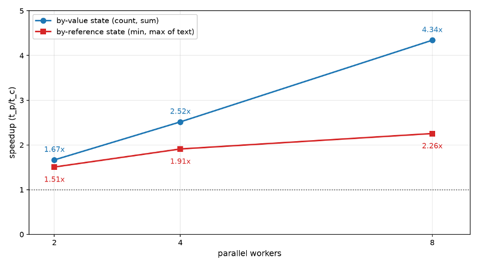Figure 1: parallel aggregate speedup scalability for uniformly distributed tuples among the groups

Negative effects on shared resources, however, usually show up sharply under access skew — on the so-called “heavy hitter” rows. Let us model the skew and generate the data so that one group gets a dominating share of the table rows, while the rest of the rows are spread evenly over the remaining groups. The number of rows (20 million) and the number of groups (1 million) are fixed; only the concentration of the “heavy hitter” group changes (fig. 2).

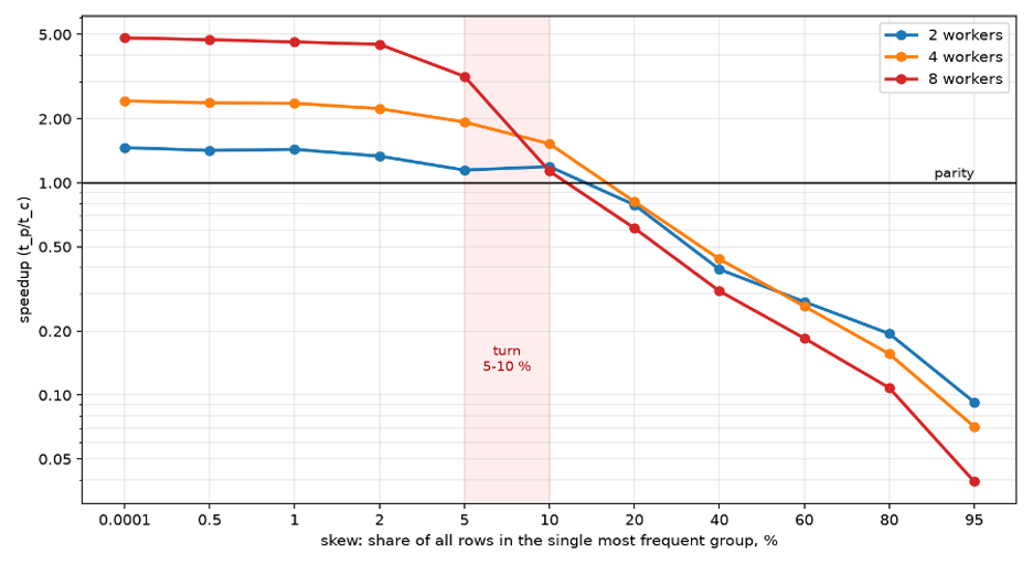Figure 2: parallel aggregate speedup behaviour with different skew factor

Up to and including 2 % the shared table wins confidently: 4.82× with eight workers on a uniform key and 4.49× at a share of 2 %. After that the advantage melts away, and between 10 and 20 % it turns into a loss, reaching 0.04× at 95 %.

So, to use parallel aggregate safely one needs good statistics on the table columns and a cost model based on MCV statistics — in order to track the frequency of the most popular values. If the largest “heavy hitter” is in the range of 5–10 % of the values, the method can still be used; for 2 % and below it will give an excellent effect.

A “heavy hitter” skew, however, is not a very practical experiment. It is much better to look at the more conventional rule of skew — 80-20. Figure 3 shows the speedup that parallel aggregate gives compared with the current master, depending on the number of workers.

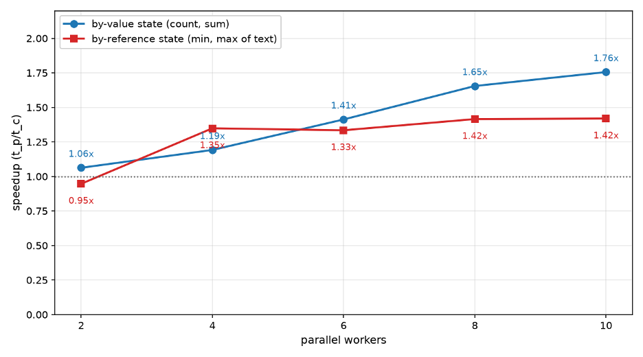Figure 3: speedup scalability for the 80-20 distribution rule

Next step – check how different distribution skew impacts the speedup. In Figure 4 we compare different variants of value density in the first 20 % of the groups in the case of the by-value (a) and by-reference (b) aggregates.

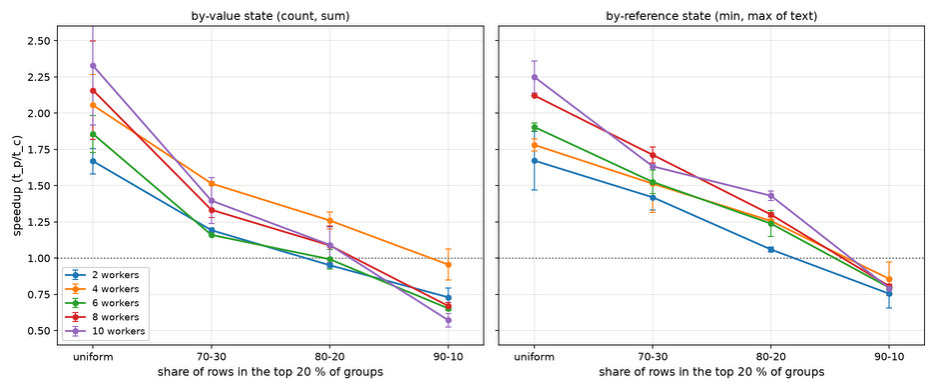Figure 4: speedup scalability dependence on distribution rule

It turns out that 80-20 is the extreme case where there is still a positive effect from parallelising: for aggregates with a by-value state it is roughly parity there already, and only by-reference still has some margin. At the same time the cost model will have to tune the number of workers needed according to the expected skew in the distribution.

One more curious observation — if we compare these two charts, it is noticeable that aggregation with a by-reference state behaves better in the parallel case than the seemingly simple by-value variant. This tells us that the current PostgreSQL core still has room to optimise the computation of aggregates by revising (or specialising) aggregation for some cases — for example, when a numeric column is declared with a known and fairly small precision, which allows all the values to fit into a fixed length int64, int128 or int256.

And finally, let us look at whether the effect of parallelising depends significantly on the number of aggregates computed per group. The following chart shows how the speedup behaves for different numbers of workers. One can see a positive effect for a number of aggregates from 4 to 12, small though it is: with eight workers the speedup grows from 4.64× on two aggregates to 5.80× on twelve. After that the effect fades away, and at 32 aggregates the speedup drops to 4.40× — lower than on two. But the very fact that this does not degrade parallel aggregate is a positive result.

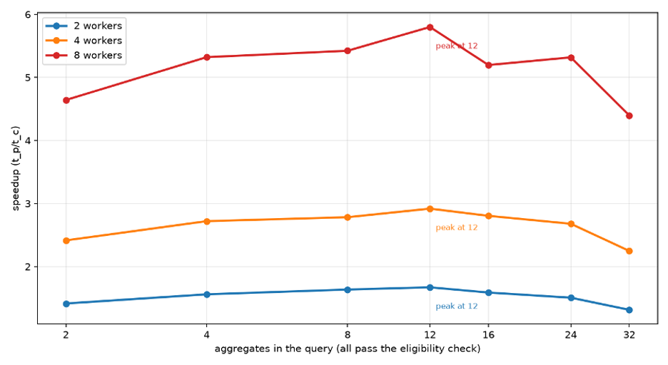Figure 5: speedup dependency on the number of aggregates to be computed

Conclusions

The main conclusion is rather trivial — the process model is the main obstacle on the way to using the shared model.

The results in favour of shared aggregation were obtained on a model with threads. A shared hash table is much cheaper in itself in that case, and the aggregate state is an ordinary object with ordinary pointers, so the code of the aggregate itself does not have to be changed at all.

In PostgreSQL the shared memory for aggregation is allocated in DSM. This means no direct pointers, no palloc, no MemoryContext, no repalloc, and no way to de-TOAST in place. So, to widen the area where parallel aggregation applies, the aggregates themselves have to be changed: at the very least, to give up the Internal state and to increase the share of aggregates whose intermediate result has a fixed size.

Besides, the solution turns out to be invasive and does not provide one of the basic optimisations — fast expression evaluation by the interpreter — and will most likely require further work on it.

The ticketing proposed in the paper removes only one kind of load, while the following main problems remain:

1. The lock is still there, and it is not free. A lock is expensive in itself, and not because of what it protects. Worse than that, LWLock is the wrong primitive for a critical section of this size: for count(*) there is a single increment under the lock, nanoseconds, while LWLockAcquire() in an unlucky case requires a context switch, microseconds.

2. There is no compiled transition program, and with it no JIT. The private path computes all the filters, all the arguments and all the transition calls with a single program from ExecBuildAggTrans(), which JIT compiles into one function. In the parallel aggregate case that path does not work: the arguments have to be computed before the lock is taken, and the transition function has to be called after it.

3. Essentially arbitrary code runs under the lock. Even on built-in types there are situations where a function (enum_cmp_internal(), for example) goes to the catalogue on certain OIDs, that is, does a table_open() and reads buffers, which potentially means one more heavy lock inside the LWLock.

Hence the conclusion: PostgreSQL pays much more for a shared mutable state than an engine with threads, and gets the same thing in return. To me, this is a solid argument in favour of partitioning.

For all that, the approach looks tempting: it noticeably reduces the memory requirements, and so postpones the start of spilling. It also reduces the number of operations by removing the Finalize stage. One more argument in favour — it can be adapted to the SetOp operator, where no parallelising is provided at all at the moment, and it will be extremely efficient for cases of simple grouping (SELECT DISTINCT, for example), where there are no aggregates and most of the problem spots of our code are simply not touched. The “Parallel Memoize” mechanism also looks tempting, although it would require some work on that mechanism, since the Memoize operator currently may evict the least recently used cache entry. So the method may be worth trying further if we agree to some compromises.

The main compromise is moving to lock-free. For that we would have to limit ourselves to fixed-width by-value states whose merge is a single atomic operation: count, sum of integers and floats. Then LWLock could be dropped altogether. That eliminates the question of lock contention, removes the serialisation mechanism for by-reference states and brings back the efficient expression interpreter.

For many uses this is a good compromise — right now some of the aggregates with an internal state (sum over bigint or numeric, for example) are rather inefficient anyway and could be optimised: in financial applications, for instance, numeric is often restricted in precision — numeric(x,y) — which is often covered by a fixed-length int128 or int256 type. But that is a topic for a separate article.